The data-entry samples and images in the
right-hand panel follow the same chronology
as what you are reading in the left-hand panel.
-----------------------------------------------
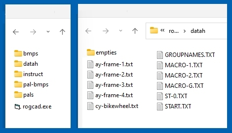
Keep all the files in the folders they came in
except where instructed otherwise, and do not
delete any folders.
Your work with RogCAD will involve just two
folders -- "empties" and "datah". Within the
datah folder, you'll want to create subfolders
named as you see fit for storing data files for
projects that are not current, otherwise you'll
end up with a lot of unrelated data files in
your working folder (the "datah" folder).
Leave all the files in the "empties" folder intact.
Copy files from that folder as needed, and place
them into the datah folder with a new name suitable
for your project.
(The data folder in RogCAD for Windows is named
"datah" to distinguish it from the "data" folder
used in RogCAD for DOS.)
There are five types of data files used in RogCAD,
and four of them come in x, y and z versions:
s-.txt ax-.txt x8-.txt cx-.txt mx-.txt
ay-.txt y8-.txt cy-.txt my-.txt
az-.txt z8-.txt cz-.txt mz-.txt
Numerical data is entered into those text files as
"standard" points : s
+ cubics
cubic elements : ax,ay,az
strings of cubics : x8,y8,z8
curves : cx,cy,cz
combination of : mx,my,mz
standard/cubics/curves
Each data file into which you've entered data is
called a "group", and you name them as you see fit.
When running RogCAD you can display any or all of
those groups on screen. Whichever group you've
most recently called for display is the "active"
group.
Projects are typically best broken into groups
such as:
s-mainshell.txt
ax-eastwindows.txt
ax-northwindows.txt
s-roof.txt
s-frontporch.txt
x8-porchrails.txt
cz-sidewalk.txt
Three other important text files that are
kept in the datah folder are:
START.TXT GROUPNAMES.TXT S-0.TXT
In START.TXT, you can edit:
default view
default color palette
default background color for CLS
fast-change views
You must enter the names of your data files
into GROUPNAMES.TXT or else RogCAD will not
recognize them.
S-0.TXT is an x-y orientation pair of lines.
RogCAD will not run if that file is removed
from the datah folder.
----------------------------------------------
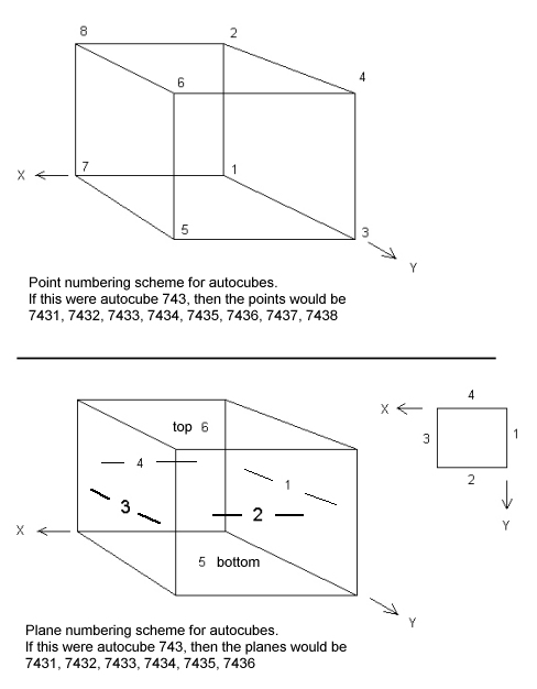
Autocubes: See right-hand panel
beginning here -->
Depending on which type of data file
you are using, autocube point numbers
begin at one of the following:
1
1001
2001
3001
4001
5001
6001
7001
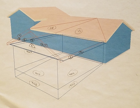
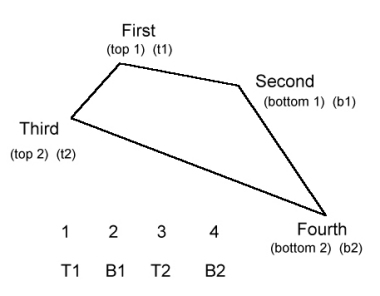
A cube has eight points, therefore autocubes have
point numbers in accordance with the following
pattern:
4001 to 4008
4011 to 4018
4021 to 4028
etc Points xxx9 and xx10
are not used.
A cube has six sides, therefore autocubes have
plane numbers in accordance with the following
pattern:
4001 to 4006
4011 to 4016
4021 to 4026
etc Planes xxx7, xxx8, xxx9 and xx10
are not used.
-------------------------------------------------
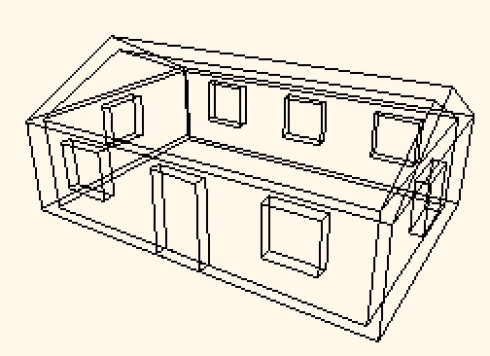
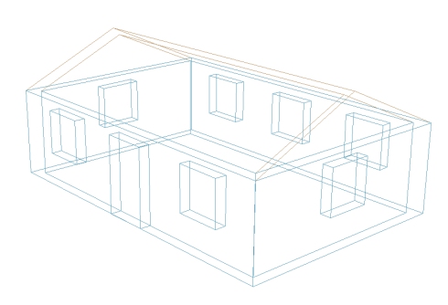
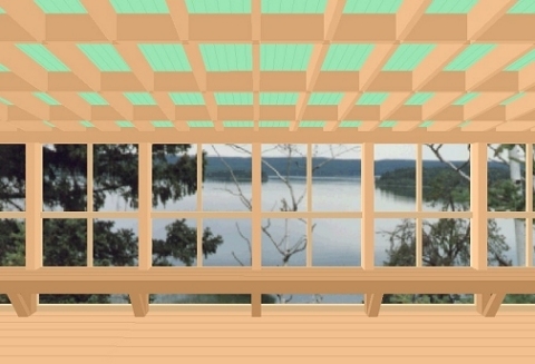
This author typically separates exterior modeling
from interior modeling, and therefore does not
typically model see-through window openings,
which are illustrated immediately to the right.
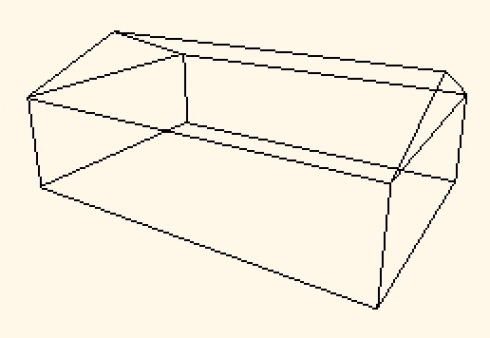
In fact, for strictly exterior modeling, exterior
walls are often just given zero thickness by
virtue of using a single autocube to define the
shell of the structure.
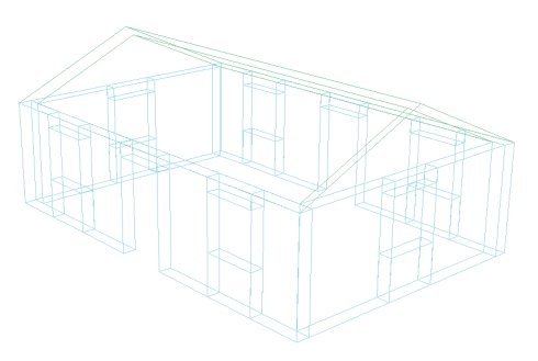
To achieve see-through window openings, one needs
to define wall sections as illustrated further
down. And that actually goes quickly, as many of
the values are simply repeated.
We'll pick up on that again after looking at the
two autocube diagrams below and to the right.
-------------------------------------------------
---->
See the autocube diagram in the right-hand panel
for the point and plane numbering scheme for
autocubes.
As you build your model, you'll probably want to
make reference sketches on which to label points
and planes of your model. It almost always comes
in handy.
 ------------------------------------------------
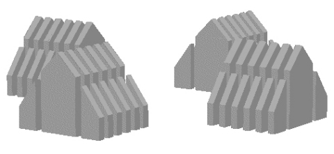
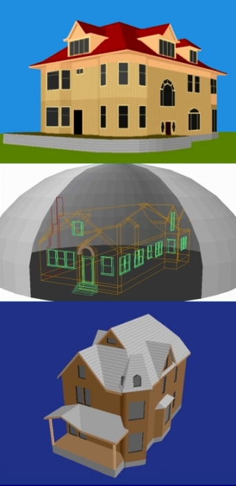
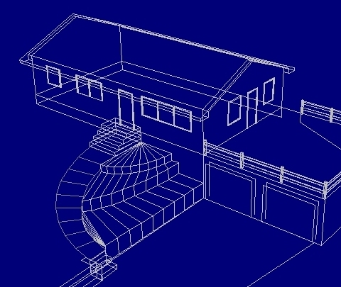
The image immediately to the right is a repeat
of the incorrect method of creating window
openings.
It would not work with the auto-surfacing
routine because the walls would get auto-surfaced
over the window openings.
Rather, the walls need to be defined in segments,
thereby creating window openings. In that case,
no autocubes are used for the window openings
themselves -- those openings exist simply as
"absence of wall".
------------------------------------------------
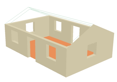
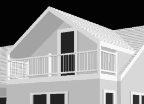
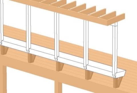
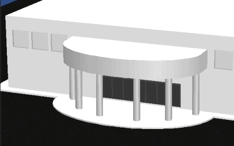
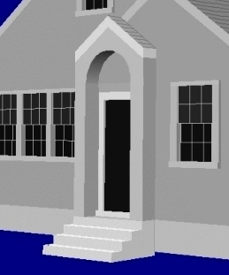
To the right is the model with those wall segments
defined, leaving voids which are regarded as
window openings.
The groups displayed here are:
s-simplehouse-3.txt
s-simpleroof-front.txt
s-simpleroof-back.txt
------------------------------------------------
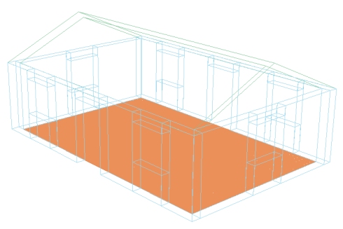
It's important to break your project into groups
so that the auto-surfacing routine will work
properly on a project-wide scope.
(The RogCAD algorithm for determining overlapping
planes is not as sophisticated as what is found
in the most expensive software. However, it's
beneficial to have your project broken in groups
for other reasons as well, so it's mostly a moot
point.)
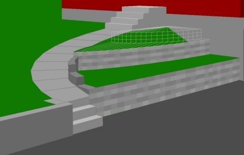
To the right we see the group named
"s-simplefloor.txt" auto-surfaced.
------------------------------------------------
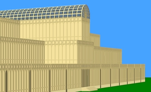
Now, to the right we see the group named
"s-simplehouse-3.txt" auto-surfaced.
------------------------------------------------
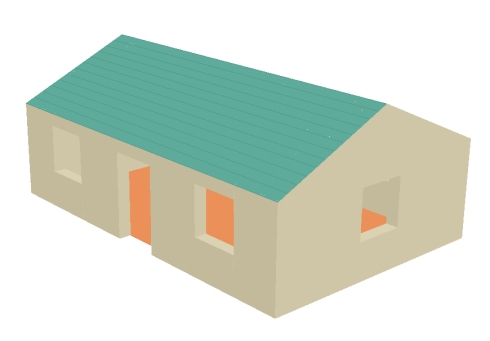
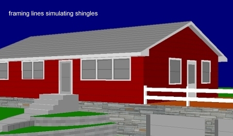
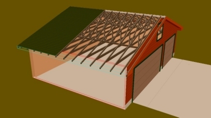
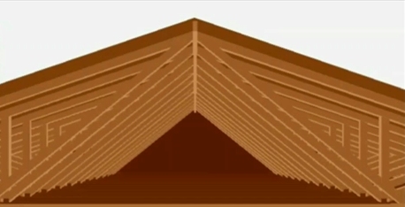
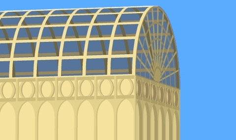
Finally, to the right we see the group named
"s-simpleroof-front" auto-surfaced.
Note that the lines representing shingles are
part of the auto-surfacing routine.
The spacing information for those lines was
entered into the AUTOFRAMING section of
st-simpleroof-front.txt.
------------------------------------------------
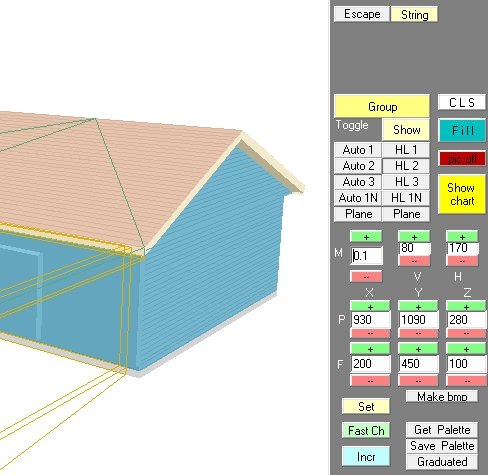
Go ahead and run rogcad[version].exe
Click on the "group" button, then select
various groups for display. It will be the most
illustrative if you select them from top to
bottom, clearing the screen after you've selected
all the groups of a cluster.
Click the CLS (clear screen) button to clear the
screen at any time.
Make sure to experiment with the view-change
buttons:
M (magnification)
V and H (vertical and horizontal shift)
P/F XYZ (perspective and focus)
---------------------------------------------
Refer to the sample project videos higher on
this page to see some button-clicking in
action.
---------------------------------------------
Below are still images that explain all the
buttons and menu items.
Below that, we'll round out part one of these
instructions by looking at data-entry more
thoroughly.
------------------------------------------------
The image immediately to the right is a repeat
of the incorrect method of creating window
openings.
It would not work with the auto-surfacing
routine because the walls would get auto-surfaced
over the window openings.
Rather, the walls need to be defined in segments,
thereby creating window openings. In that case,
no autocubes are used for the window openings
themselves -- those openings exist simply as
"absence of wall".
------------------------------------------------
To the right is the model with those wall segments
defined, leaving voids which are regarded as
window openings.
The groups displayed here are:
s-simplehouse-3.txt
s-simpleroof-front.txt
s-simpleroof-back.txt
------------------------------------------------
It's important to break your project into groups
so that the auto-surfacing routine will work
properly on a project-wide scope.
(The RogCAD algorithm for determining overlapping
planes is not as sophisticated as what is found
in the most expensive software. However, it's
beneficial to have your project broken in groups
for other reasons as well, so it's mostly a moot
point.)
To the right we see the group named
"s-simplefloor.txt" auto-surfaced.
------------------------------------------------
Now, to the right we see the group named
"s-simplehouse-3.txt" auto-surfaced.
------------------------------------------------
Finally, to the right we see the group named
"s-simpleroof-front" auto-surfaced.
Note that the lines representing shingles are
part of the auto-surfacing routine.
The spacing information for those lines was
entered into the AUTOFRAMING section of
st-simpleroof-front.txt.
------------------------------------------------
Go ahead and run rogcad[version].exe
Click on the "group" button, then select
various groups for display. It will be the most
illustrative if you select them from top to
bottom, clearing the screen after you've selected
all the groups of a cluster.
Click the CLS (clear screen) button to clear the
screen at any time.
Make sure to experiment with the view-change
buttons:
M (magnification)
V and H (vertical and horizontal shift)
P/F XYZ (perspective and focus)
---------------------------------------------
Refer to the sample project videos higher on
this page to see some button-clicking in
action.
---------------------------------------------
Below are still images that explain all the
buttons and menu items.
Below that, we'll round out part one of these
instructions by looking at data-entry more
thoroughly.
|
 Extremely simple house:
See s-simplehouse-1.txt
STANDARD: point numbers
1 0,0,0 followed by their
2 0,0,8 x y z values
3 0,30,0
4 0,30,8
5 20,30,0
6 20,30,8
7 20,0,0
8 20,0,8
9 10,0,12
10 10,30,12
999 999,999,999 end of data read
Use spaces or commas to separate
numerical information.
Connect the points defined above,
or else RogCAD won't recognize the points:
LINEG1:
1,2 3,4 5,6 7,8 1,3
3,5 5,7 7,1 2,4 4,6
6,8 8,2 8,9 9,2 6,10
10,4 9,10
999,999
Extremely simple house:
See s-simplehouse-1.txt
STANDARD: point numbers
1 0,0,0 followed by their
2 0,0,8 x y z values
3 0,30,0
4 0,30,8
5 20,30,0
6 20,30,8
7 20,0,0
8 20,0,8
9 10,0,12
10 10,30,12
999 999,999,999 end of data read
Use spaces or commas to separate
numerical information.
Connect the points defined above,
or else RogCAD won't recognize the points:
LINEG1:
1,2 3,4 5,6 7,8 1,3
3,5 5,7 7,1 2,4 4,6
6,8 8,2 8,9 9,2 6,10
10,4 9,10
999,999
 Below, fewer standard points are defined,
while autocubes are used to define an inner and
outer shell and to create simple window openings.
However, THIS IS NOT THE CORRECT METHOD for
creating window openings, and is included as
a simple first example of using autocubes.
The correct method for creating window openings
is in the example that follows beneath this one.
--------------------------------------------------
See s-simplehouse-2.txt
STANDARD:
1 10 1 12
2 10 29 12
3 10 0 12.5
4 10 30 12.5
999 999,999,999
LINEG1:
1,2 3,4
1,4002 1,4008 2,4004 2,4006
3,4012 3,4018 4,4014 4,4016
999,999
NOTE that we can connect standard points to
autocube points, and we can define planes in
the same manner.
start rotation index
point min xyz max xyz and base color
----- ------- ------- --------------
AUTOCUBE400:
4001 1,1,0 19,29,8 0,5
4011 0,0,0 20,30,8 0,5
4021 8,0,3 12,1,7 0,5
4031 0,4,3 1,8,7 0,5
4041 0,13,3 1,17,7 0,5
4051 0,22,3 1,26,7 0,5
4061 8,29,3 12,30,7 0,5
4071 19,4,3 20,8,7 0,5
4081 19,13,0 20,17,7 0,5
4091 19,22,3 20,26,7 0,5
999 999,999,999 999,999,999 0,0
Rotation indexes and base colors have been
left at the default value for now.
Below, fewer standard points are defined,
while autocubes are used to define an inner and
outer shell and to create simple window openings.
However, THIS IS NOT THE CORRECT METHOD for
creating window openings, and is included as
a simple first example of using autocubes.
The correct method for creating window openings
is in the example that follows beneath this one.
--------------------------------------------------
See s-simplehouse-2.txt
STANDARD:
1 10 1 12
2 10 29 12
3 10 0 12.5
4 10 30 12.5
999 999,999,999
LINEG1:
1,2 3,4
1,4002 1,4008 2,4004 2,4006
3,4012 3,4018 4,4014 4,4016
999,999
NOTE that we can connect standard points to
autocube points, and we can define planes in
the same manner.
start rotation index
point min xyz max xyz and base color
----- ------- ------- --------------
AUTOCUBE400:
4001 1,1,0 19,29,8 0,5
4011 0,0,0 20,30,8 0,5
4021 8,0,3 12,1,7 0,5
4031 0,4,3 1,8,7 0,5
4041 0,13,3 1,17,7 0,5
4051 0,22,3 1,26,7 0,5
4061 8,29,3 12,30,7 0,5
4071 19,4,3 20,8,7 0,5
4081 19,13,0 20,17,7 0,5
4091 19,22,3 20,26,7 0,5
999 999,999,999 999,999,999 0,0
Rotation indexes and base colors have been
left at the default value for now.
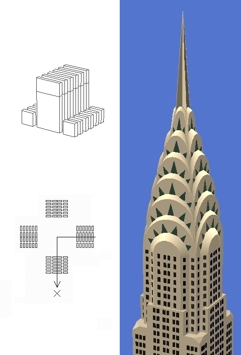
 Again, this is NOT the manner in which autocubes
are typically combined to build architectural
structures. It's for simple illustration.
Typically, you'll want to define autocubes in
a manner that will facilitate successful
sorting of planes for auto-surfacing
(automatic plane coloring).
That's covered in the example beneath this
autocube diagram:
Again, this is NOT the manner in which autocubes
are typically combined to build architectural
structures. It's for simple illustration.
Typically, you'll want to define autocubes in
a manner that will facilitate successful
sorting of planes for auto-surfacing
(automatic plane coloring).
That's covered in the example beneath this
autocube diagram:
 incorrect window openings:
 correct window openings:
 --------------------------------------------------
|
 ------------------------------------------------------------------------------------------------
The enter key on your keyboard has no functionality in RogCAD.
You must use the enter buttons provided on the user interface.
Use your mouse to highlight and delete anything in the text boxes
as needed. These little text boxes work just like any text displayed
by Windows.
------------------------------------------------------------------------------------------------
------------------------------------------------------------------------------------------------
The enter key on your keyboard has no functionality in RogCAD.
You must use the enter buttons provided on the user interface.
Use your mouse to highlight and delete anything in the text boxes
as needed. These little text boxes work just like any text displayed
by Windows.
------------------------------------------------------------------------------------------------
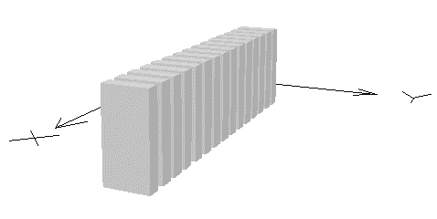
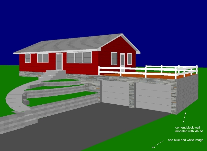
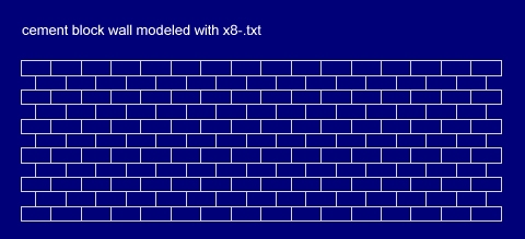
 Here are examples of autocubes repeated along the x axis from an x8-.txt data file.
As with single autocubes, we specify minimum xyz values
and maximum xyz values.
The spacing dictates just that - how to space those repeating autocubes.
The units of measure are the same as used for xyz values.
First we see autocube block 200, meaning points begin at 2001.
End cube 208 has points 2081 to 2088.
Eight cubics will be drawn, spaced out along the x axis every 18 inches.
Below that we see block 300, with points beginning at 3001.
Seven cubics will be drawn, spaced out along the x axis every 18 inches.
We say "cubics" even though in this particular case, those cubics
are completely flat, two-dimensional, since we used 0 for both the
minimum and maximum value for z.
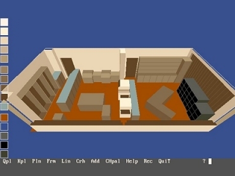
These flat cubics are 9" x 9" floor tiles, with a white and black
checker-board pattern. By using additional blocks, we quickly tile
an entire room:
See the image of the kitchen
near the top of this document.
The final two values are rotation index and base color.
If you do not subject this data to a rotation by way of using
the transformation routines, then 0 is the correct value.
90 degree => rotation index of 1
180 degree => rotation index of 2
270 degree => rotation index of 3
Other degrees => whatever works best: 0, 1, 2 or 3.
The rotation index and base color work in
conjunction with the autosurfacing routine.
x y z x y z spacing end plane rot,col
-------------------------------------------------------------------------
(201 - 299)
AUTOCUBE200:
0 9 0 9 18 0 18 208 0,1
(301 - 399)
AUTOCUBE300:
9 9 0 18 18 0 18 307 0,1
-------------------------------------------------------------------------
Cubics repeated along an axis, then mitered and tilted with transformations:
Here are examples of autocubes repeated along the x axis from an x8-.txt data file.
As with single autocubes, we specify minimum xyz values
and maximum xyz values.
The spacing dictates just that - how to space those repeating autocubes.
The units of measure are the same as used for xyz values.
First we see autocube block 200, meaning points begin at 2001.
End cube 208 has points 2081 to 2088.
Eight cubics will be drawn, spaced out along the x axis every 18 inches.
Below that we see block 300, with points beginning at 3001.
Seven cubics will be drawn, spaced out along the x axis every 18 inches.
We say "cubics" even though in this particular case, those cubics
are completely flat, two-dimensional, since we used 0 for both the
minimum and maximum value for z.
These flat cubics are 9" x 9" floor tiles, with a white and black
checker-board pattern. By using additional blocks, we quickly tile
an entire room:
See the image of the kitchen
near the top of this document.
The final two values are rotation index and base color.
If you do not subject this data to a rotation by way of using
the transformation routines, then 0 is the correct value.
90 degree => rotation index of 1
180 degree => rotation index of 2
270 degree => rotation index of 3
Other degrees => whatever works best: 0, 1, 2 or 3.
The rotation index and base color work in
conjunction with the autosurfacing routine.
x y z x y z spacing end plane rot,col
-------------------------------------------------------------------------
(201 - 299)
AUTOCUBE200:
0 9 0 9 18 0 18 208 0,1
(301 - 399)
AUTOCUBE300:
9 9 0 18 18 0 18 307 0,1
-------------------------------------------------------------------------
Cubics repeated along an axis, then mitered and tilted with transformations:
 Creating mitered framing members by skewing
cubics with STEP10TRANSLATE snippet:
Creating mitered framing members by skewing
cubics with STEP10TRANSLATE snippet:


 macro-a, continued from left-hand panel:
In the snippets that follow you'll see:
------------------------------------------
s
steps (the front steps of a house)
s refers to s type of group.
s-steps.txt is the group thus referenced.
------------------------------------------
The number entered into the AUTOSURFACE
function corresponds to either Auto1, Auto2,
Auto3, Auto1N, HL1, HL2, HL3 or HL1N
as used in the RogCAD interface at run-time.
1 = Auto1 2 = Auto2 3 = Auto3 7 = Auto1N
4 = HL1 5 = HL2 6 = HL3 10 = HL1N
Auto1N and HL1N can be used for narrow planes.
The object might get surfaced a couple seconds
faster.
Lightest and darkest side for auto-surfacing
is set in the data-files.
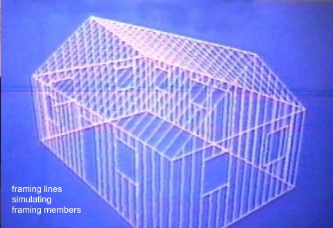
The other additional function in macro-a is
the HIDESHOW function. When the value is
set to 0, the wireframe lines of that data group
will not display. That setting is by far the
most common, since wireframe lines would defeat
the purpose of surface-modeling. However,
situations do come up where it's actually
desirable to display the wireframe lines for
a data group as part of the finished model.
MACROGROUPS:
400,2000
=======================================nextgroup
s
steps
----------------------------AUTOSURFACE
2
----------------------------SJK
0,0,0,0,0
----------------------------PLANES
0,0
----------------------------CROSSHATCH
0,0,0,0,0,0
----------------------------FRAMINGLINES
0,0,0,0,0,0
----------------------------HIDESHOW
0
----------------------------LINES
0,0,0
=======================================nextgroup
cz
walk
----------------------------AUTOSURFACE
0
----------------------------SJK
1 9 1 4 0
0,0,0,0,0
----------------------------PLANES
0,0
----------------------------CROSSHATCH
0,0,0,0,0,0
----------------------------FRAMINGLINES
0,0,0,0,0,0
----------------------------HIDESHOW
1
----------------------------LINES
0,0,0
=======================================nextgroup
cz
rock
----------------------------AUTOSURFACE
0
----------------------------SJK
121 129 1 10 0
21 29 1 10 0
1 9 1 6 0
61 70 1 10 0
41 49 1 6 0
101 109 1 10 0
81 89 1 6 0
0,0,0,0,0
----------------------------PLANES
0,0
----------------------------CROSSHATCH
1 11 10 20 18 7
1 10 11 20 6 5
41 51 50 60 16 7
41 50 51 60 5 5
81 91 90 100 11 7
81 90 91 100 3 5
0,0,0,0,0,0
----------------------------FRAMINGLINES
0,0,0,0,0,0
----------------------------HIDESHOW
0
----------------------------LINES
0,0,0
=======================================nextgroup
s
lsteps
----------------------------AUTOSURFACE
2
----------------------------SJK
0,0,0,0,0
----------------------------PLANES
0,0
----------------------------CROSSHATCH
0,0,0,0,0,0
----------------------------FRAMINGLINES
233 234 235 236 9 7
233 235 234 236 6 6
0,0,0,0,0,0
----------------------------HIDESHOW
0
----------------------------LINES
0,0,0
GROUPEND
------------------------------------------------
macro-a, continued from left-hand panel:
In the snippets that follow you'll see:
------------------------------------------
s
steps (the front steps of a house)
s refers to s type of group.
s-steps.txt is the group thus referenced.
------------------------------------------
The number entered into the AUTOSURFACE
function corresponds to either Auto1, Auto2,
Auto3, Auto1N, HL1, HL2, HL3 or HL1N
as used in the RogCAD interface at run-time.
1 = Auto1 2 = Auto2 3 = Auto3 7 = Auto1N
4 = HL1 5 = HL2 6 = HL3 10 = HL1N
Auto1N and HL1N can be used for narrow planes.
The object might get surfaced a couple seconds
faster.
Lightest and darkest side for auto-surfacing
is set in the data-files.
The other additional function in macro-a is
the HIDESHOW function. When the value is
set to 0, the wireframe lines of that data group
will not display. That setting is by far the
most common, since wireframe lines would defeat
the purpose of surface-modeling. However,
situations do come up where it's actually
desirable to display the wireframe lines for
a data group as part of the finished model.
MACROGROUPS:
400,2000
=======================================nextgroup
s
steps
----------------------------AUTOSURFACE
2
----------------------------SJK
0,0,0,0,0
----------------------------PLANES
0,0
----------------------------CROSSHATCH
0,0,0,0,0,0
----------------------------FRAMINGLINES
0,0,0,0,0,0
----------------------------HIDESHOW
0
----------------------------LINES
0,0,0
=======================================nextgroup
cz
walk
----------------------------AUTOSURFACE
0
----------------------------SJK
1 9 1 4 0
0,0,0,0,0
----------------------------PLANES
0,0
----------------------------CROSSHATCH
0,0,0,0,0,0
----------------------------FRAMINGLINES
0,0,0,0,0,0
----------------------------HIDESHOW
1
----------------------------LINES
0,0,0
=======================================nextgroup
cz
rock
----------------------------AUTOSURFACE
0
----------------------------SJK
121 129 1 10 0
21 29 1 10 0
1 9 1 6 0
61 70 1 10 0
41 49 1 6 0
101 109 1 10 0
81 89 1 6 0
0,0,0,0,0
----------------------------PLANES
0,0
----------------------------CROSSHATCH
1 11 10 20 18 7
1 10 11 20 6 5
41 51 50 60 16 7
41 50 51 60 5 5
81 91 90 100 11 7
81 90 91 100 3 5
0,0,0,0,0,0
----------------------------FRAMINGLINES
0,0,0,0,0,0
----------------------------HIDESHOW
0
----------------------------LINES
0,0,0
=======================================nextgroup
s
lsteps
----------------------------AUTOSURFACE
2
----------------------------SJK
0,0,0,0,0
----------------------------PLANES
0,0
----------------------------CROSSHATCH
0,0,0,0,0,0
----------------------------FRAMINGLINES
233 234 235 236 9 7
233 235 234 236 6 6
0,0,0,0,0,0
----------------------------HIDESHOW
0
----------------------------LINES
0,0,0
GROUPEND
------------------------------------------------
 ------------------------------------------------
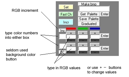
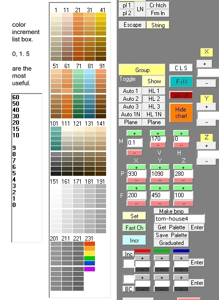
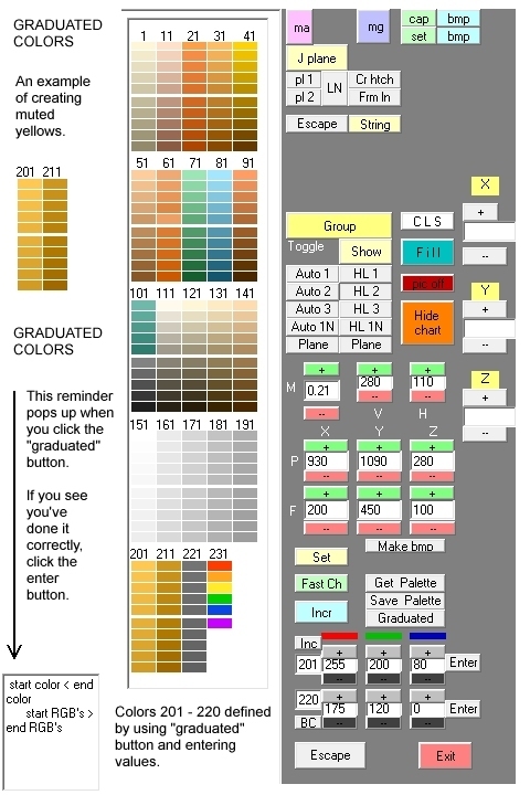 RogCAD now has a Grad 150 button on its
interface. It works like the Graduated
button, except that you enter just high-
value numbers for red, green, blue in the
top red/green/blue row.
Graduated colors will fill the chart from
colors 1 to 150.
RogCAD now has a Grad 150 button on its
interface. It works like the Graduated
button, except that you enter just high-
value numbers for red, green, blue in the
top red/green/blue row.
Graduated colors will fill the chart from
colors 1 to 150.
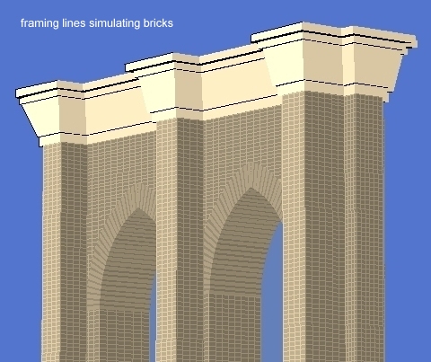
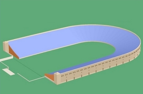
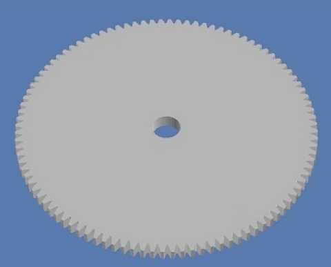
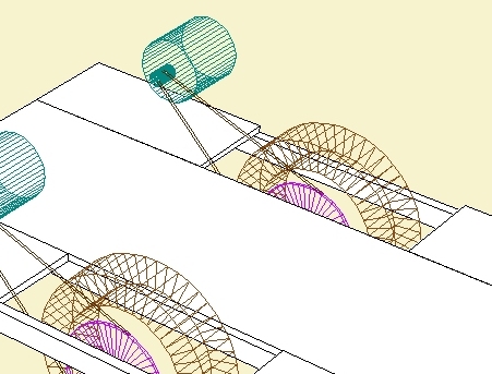
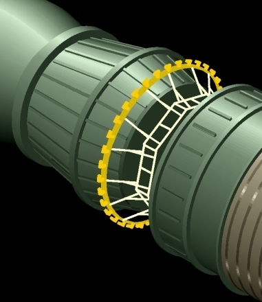
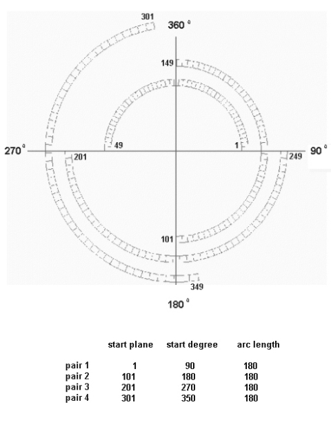 You'll notice in the images above and below that
each arc consists of two long curved parallel
lines and 50 short lines connecting them. What
we really have are 49 small rectangles simulating
a curve. Each (double) curve consists of 100
data points, regardless of the arc length.
You can specify any even number of points for
your curve.
The number of planes generated will be half the
number of points you specify minus 1.
More on that further down.
These points, lines and planes are generated
automatically by the curve routine. You just
specify the start degree, the arc length, two
radii, the offset, and the modifiers (which
consist of three numbers).
If the radii (y and z in this case, since the
curve is wrapping around the x-axis in cx-.txt)
are equal, then you will generate a perfectly
circular curve.
If the radii are not equal, you will generate an
elliptical curve.
Each curve must consist of two curve-lines, though
they need not be uniform within that pair in any
manner:
You can vary the radius between the top line and
the bottom line, or you can vary the offset, or
both, depending on what architectural element you
are building.
You can generate a limitless variety of irregular
curved surfaces.
You can also make the two curve-lines (top line
and bottom line) identical, thereby effectively
generating a single lined curve if you need to.
You can terminate the data read by placing the
999 beneath whichever line pair you wish to be
your last.
You'll notice in the images above and below that
each arc consists of two long curved parallel
lines and 50 short lines connecting them. What
we really have are 49 small rectangles simulating
a curve. Each (double) curve consists of 100
data points, regardless of the arc length.
You can specify any even number of points for
your curve.
The number of planes generated will be half the
number of points you specify minus 1.
More on that further down.
These points, lines and planes are generated
automatically by the curve routine. You just
specify the start degree, the arc length, two
radii, the offset, and the modifiers (which
consist of three numbers).
If the radii (y and z in this case, since the
curve is wrapping around the x-axis in cx-.txt)
are equal, then you will generate a perfectly
circular curve.
If the radii are not equal, you will generate an
elliptical curve.
Each curve must consist of two curve-lines, though
they need not be uniform within that pair in any
manner:
You can vary the radius between the top line and
the bottom line, or you can vary the offset, or
both, depending on what architectural element you
are building.
You can generate a limitless variety of irregular
curved surfaces.
You can also make the two curve-lines (top line
and bottom line) identical, thereby effectively
generating a single lined curve if you need to.
You can terminate the data read by placing the
999 beneath whichever line pair you wish to be
your last.
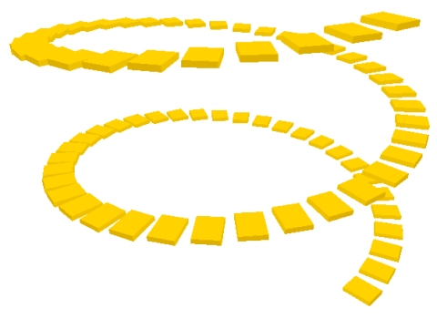
 Curve painting
Keep in mind that RogCAD's auto-surfacing
routine will paint your curves for you with
smooth gradient lighting.
The Auto C button activates it at run-time.
You edit DARKESTCOLOR in the cx,cy,cz,mx,my,mz
data files by specifying a color number. Your
curves will be given smooth gradient lighting,
with the closest plane based on perspective
receiving the lightest color.
But there are plenty of circumstances where
you will prefer to use the macro-files,
or -- when testing your design -- the string
button on the user-interface.
The string button is the equivalent of the
SJK routine in macro-g.txt and the macro-a files.
The methods described below might seem a bit
slow, but once you've entered the numbers into
macro-g.txt and/or macro-a.txt, you can display
the curves in surfaced form with the click of
a button.
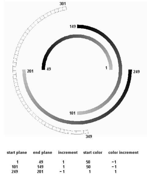
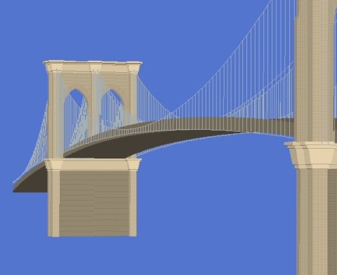
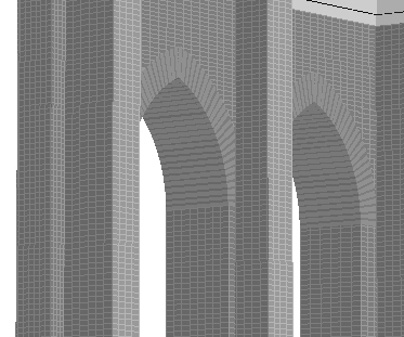
The above image shows the same simple arcs of the
previous image after being auto-surfaced using
the string routine manually or as part of
macro-g.txt or a macro-a text-file.
You can of course paint the planes of a curved
surface one at a time, and you might find
yourself doing that for a plane here and there
on the user-interface while testing your design.
But of course the simplest way to paint an arc
or a portion thereof, is to use the string
(or SJK) method.
See the SJK section higher in this document,
just above the TRANSFORMATIONS section, to review
the methodology.
Devote enough of your color palette to allow for
the number of points (and therefore planes) you
are specifying for your curve data.
You use the "graduated" button on the user-
interface to create a smooth gradient differential
for your palette over your specified range of
color numbers.
Typically, when shading a full circle object
using the string button (or SJK routine), one
would shade the planes furthest away first,
covering 180 degrees, then the planes that are
nearest.
And recall that a color increment of 0 will color
all the planes the same color.
Curve painting
Keep in mind that RogCAD's auto-surfacing
routine will paint your curves for you with
smooth gradient lighting.
The Auto C button activates it at run-time.
You edit DARKESTCOLOR in the cx,cy,cz,mx,my,mz
data files by specifying a color number. Your
curves will be given smooth gradient lighting,
with the closest plane based on perspective
receiving the lightest color.
But there are plenty of circumstances where
you will prefer to use the macro-files,
or -- when testing your design -- the string
button on the user-interface.
The string button is the equivalent of the
SJK routine in macro-g.txt and the macro-a files.
The methods described below might seem a bit
slow, but once you've entered the numbers into
macro-g.txt and/or macro-a.txt, you can display
the curves in surfaced form with the click of
a button.
The above image shows the same simple arcs of the
previous image after being auto-surfaced using
the string routine manually or as part of
macro-g.txt or a macro-a text-file.
You can of course paint the planes of a curved
surface one at a time, and you might find
yourself doing that for a plane here and there
on the user-interface while testing your design.
But of course the simplest way to paint an arc
or a portion thereof, is to use the string
(or SJK) method.
See the SJK section higher in this document,
just above the TRANSFORMATIONS section, to review
the methodology.
Devote enough of your color palette to allow for
the number of points (and therefore planes) you
are specifying for your curve data.
You use the "graduated" button on the user-
interface to create a smooth gradient differential
for your palette over your specified range of
color numbers.
Typically, when shading a full circle object
using the string button (or SJK routine), one
would shade the planes furthest away first,
covering 180 degrees, then the planes that are
nearest.
And recall that a color increment of 0 will color
all the planes the same color.

 Here is the code snippet that generated the image
to the left.
number
of radius offset weight
points start,arc Z Y X,Y,Z left,inc stretch
100
90 180 10,10 0,0,0 0,0 0
90 180 11,11 0,0,0 0,0 0
100
180 180 13,13 0,0,0 0,0 0
180 180 14,14 0,0,0 0,0 0
100
270 180 16,16 0,0,0 0,0 0
270 180 17,17 0,0,0 0,0 0
100
350 180 19,19 0,0,0 0,0 0
350 180 20,20 0,0,0 0,0 0
999
360 180 0,0 0,0,0 0,0 0
360 180 0,0 0,0,0 0,0 0
number of points/pair must be even number.
number of planes/pair = (num of points / 2) - 1
Example:
num of pts point numbers plane numbers
---------- ------------- -------------
20 1-20 1-9
20 21-40 21-29
34 41-74 41-56
12 75-86 75-79
8000 max
Up to 400 pairs (you'll never come close).
Obviously, it's advantageous to use multiples
of ten for number of points if you want to
get a handle on what the plane numbers are.
There can be circumstances where you'll want
to vary the number of points in the sections
(pairs of curve lines) within a data file.
But to make things easy to keep track of,
it's best to use the same number of points
throughout a data file.
Here is the code snippet that generated the image
to the left.

number
of                radius   offset  weight
points  start,arc  Z  Y    X,Y,Z  left,inc  stretch

100
         90  180   10,10   0,0,0      0,0       0
         90  180   11,11   0,0,0      0,0       0
100
        180  180   13,13   0,0,0      0,0       0
        180  180   14,14   0,0,0      0,0       0
100
        270  180   16,16   0,0,0      0,0       0
        270  180   17,17   0,0,0      0,0       0
100
        350  180   19,19   0,0,0      0,0       0
        350  180   20,20   0,0,0      0,0       0
999
        360  180    0,0    0,0,0      0,0       0
        360  180    0,0    0,0,0      0,0       0


number of points/pair must be even number.

number of planes/pair = (num of points / 2) - 1

Example:

num of pts   point numbers    plane numbers
----------   -------------    -------------
20            1-20             1-9
20           21-40            21-29
34           41-74            41-56
12           75-86            75-79

              8000 max

Up to 400 pairs (you'll never come close).

Obviously, it's advantageous to use multiples
of ten for number of points if you want to
get a handle on what the plane numbers are.

There can be circumstances where you'll want
to vary the number of points in the sections
(pairs of curve lines) within a data file.

But to make things easy to keep track of,
it's best to use the same number of points
throughout a data file.
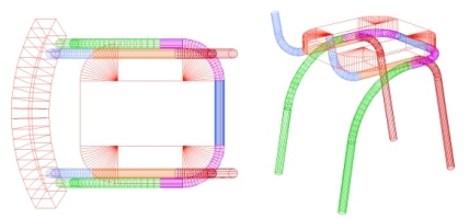
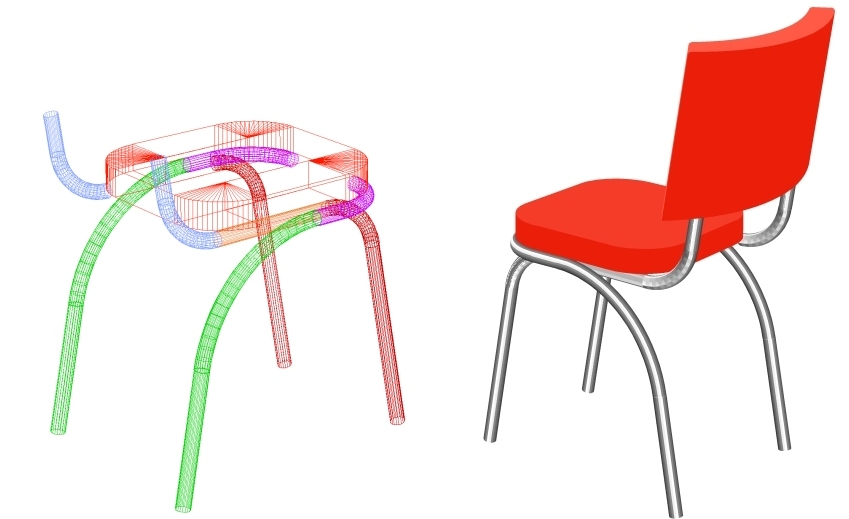 chair-back
number radius offset weight
of --------- ------------ --------
points start arc X Y X Y Z left inc stretch
CURVDATA:
40
295.9 51.8 17.75 17.75 7 17.05 32.5 0 0 0
299 58 19.5 19.5 7 17.05 32.5 0 0 0
40
299 58 19.5 19.5 7 17.05 32.5 0 0 0
299 58 19.5 19.5 7 17.05 20.75 0 0 0
40
299 58 19.5 19.5 7 17.05 20.75 0 0 0
295.9 51.8 17.75 17.75 7 17.05 20.75 0 0 0
40
295.9 51.8 17.75 17.75 7 17.05 20.75 0 0 0
295.9 51.8 17.75 17.75 7 17.05 32.5 0 0 0
999
0 90 10 10 0 0 0 0 0 0
0 90 10 10 0 0 0 0 0 0
chair-back
number radius offset weight
of --------- ------------ --------
points start arc X Y X Y Z left inc stretch
CURVDATA:
40
295.9 51.8 17.75 17.75 7 17.05 32.5 0 0 0
299 58 19.5 19.5 7 17.05 32.5 0 0 0
40
299 58 19.5 19.5 7 17.05 32.5 0 0 0
299 58 19.5 19.5 7 17.05 20.75 0 0 0
40
299 58 19.5 19.5 7 17.05 20.75 0 0 0
295.9 51.8 17.75 17.75 7 17.05 20.75 0 0 0
40
295.9 51.8 17.75 17.75 7 17.05 20.75 0 0 0
295.9 51.8 17.75 17.75 7 17.05 32.5 0 0 0
999
0 90 10 10 0 0 0 0 0 0
0 90 10 10 0 0 0 0 0 0
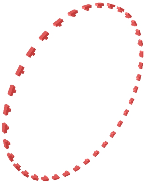
 -------------------------------------------------
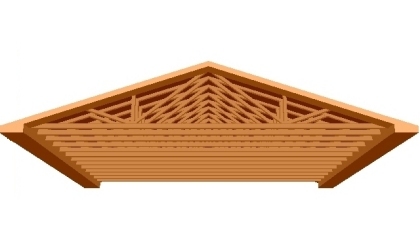
hub1
-------------------------------------------------
hub1
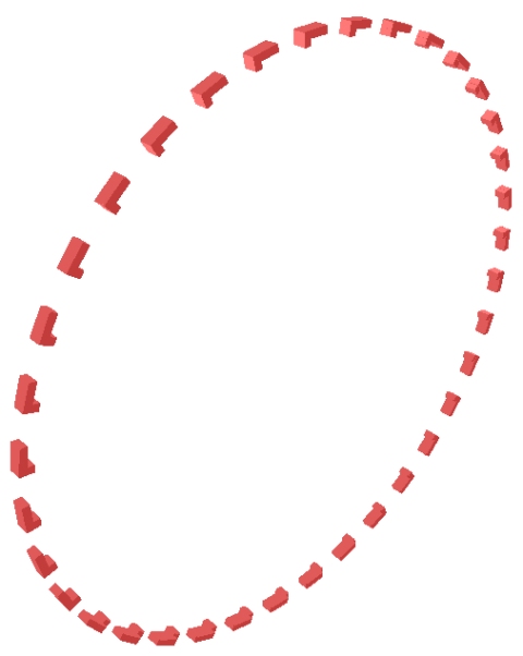
 -------------------------------------------------
hub2
-------------------------------------------------
hub2
 -------------------------------------------------
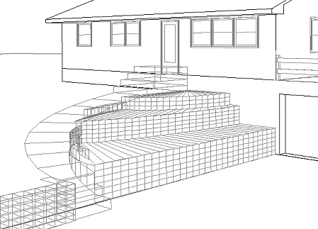
steps
-------------------------------------------------
steps
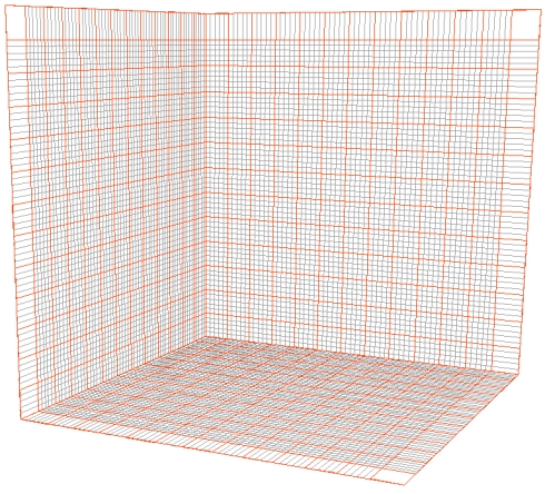 We use the x8,y8,z8 data files to create custom
grids by which to analyze the positioning and
sizing of the elements of our project. Using
multi-color lines within the grids and within
your objects makes for easy distinctions and
measurements.
x8-X-Y-GRID.txt, x8-X-Z-GRID.txt, x8-Y-Z-GRID.txt
are general-purpose grids included in the sample
datah folders. To increase or decrease their
magnification, you could simply use a RESIZE
snippet. Though to avoid confusion, you might
want to change the values in the AUTOCUBES
sections.
It's definitely handy to use the TRANSLATE,
XROTATETRANSLATE, YROTATETRANSLATE,
ZROTATETRANSLATE snippets to shift grids around
from time to time, possibly saving various
incarnations of your grids using various names.
Plan views and side elevation views of your
model are obtained by choosing the x / y / z
"full" or "zoom" views from the "fast change"
button's list box. It's useful, especially in
conjunction with grids as a background, for
showing you just what values are needed for
rotating and sliding your objects using the
transormation snippets.
You can also use a RESIZE snippet to create a
plan drawing by setting all the z values in your
data file to zero. Similarly, you can create
side elevation views by setting x or y values
to zero.
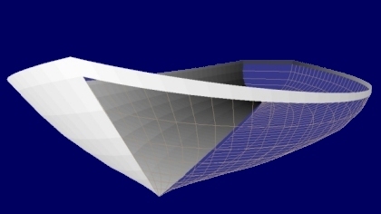
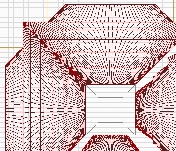
You can take your perspective point inside an
object. Some errant lines can occassionally
appear in such case (a quirk inherent in the
programming language used to create RogCAD).
Try shifting your perspective a bit. If errant
lines persist, you can simulate an inside view
by placing your perspective point outside the
object and adjusting your magnification and
focal point to create the same view as if you
were truly inside. RogCAD allows for wide
angle lens shots by bringing the perspective
point in close and selecting a focal point and
magnification to create the desired effect.
We use the x8,y8,z8 data files to create custom
grids by which to analyze the positioning and
sizing of the elements of our project. Using
multi-color lines within the grids and within
your objects makes for easy distinctions and
measurements.
x8-X-Y-GRID.txt, x8-X-Z-GRID.txt, x8-Y-Z-GRID.txt
are general-purpose grids included in the sample
datah folders. To increase or decrease their
magnification, you could simply use a RESIZE
snippet. Though to avoid confusion, you might
want to change the values in the AUTOCUBES
sections.
It's definitely handy to use the TRANSLATE,
XROTATETRANSLATE, YROTATETRANSLATE,
ZROTATETRANSLATE snippets to shift grids around
from time to time, possibly saving various
incarnations of your grids using various names.
Plan views and side elevation views of your
model are obtained by choosing the x / y / z
"full" or "zoom" views from the "fast change"
button's list box. It's useful, especially in
conjunction with grids as a background, for
showing you just what values are needed for
rotating and sliding your objects using the
transormation snippets.
You can also use a RESIZE snippet to create a
plan drawing by setting all the z values in your
data file to zero. Similarly, you can create
side elevation views by setting x or y values
to zero.
You can take your perspective point inside an
object. Some errant lines can occassionally
appear in such case (a quirk inherent in the
programming language used to create RogCAD).
Try shifting your perspective a bit. If errant
lines persist, you can simulate an inside view
by placing your perspective point outside the
object and adjusting your magnification and
focal point to create the same view as if you
were truly inside. RogCAD allows for wide
angle lens shots by bringing the perspective
point in close and selecting a focal point and
magnification to create the desired effect.